2.3. Interferometric data sets
In SMILI, interfreometric data sets are handle by uvdata module. Here, we show a basic usage of uvdata module using a VLBA data set of 3C 273 at 43 GHz of the Boston University Blazar Group.
[1]:
%matplotlib inline
from smili import uvdata, imdata, imaging, util

# for plotting
import matplotlib.pyplot as plt
2.3.1. Load/Save uvfits file and select a stokes parameter
SMILI can load a single-source uvfits files generated by eht-imaging library, AIPS task SPLIT, and DIFMAP. uvdata.UVFITS object handles data loaded from UVFITS file.
[14]:
# Include class to load uvfits data
uvfits = uvdata.UVFITS("3C273DEC16.UVP")
Filename: 3C273DEC16.UVP
No.    Name      Ver    Type      Cards   Dimensions   Format
  0  PRIMARY       1 GroupsHDU      155   (3, 4, 1, 4, 1, 1)   float32   1913 Groups  7 Parameters
  1  AIPS NX       1 BinTableHDU     31   8R x 7C   [1E, 1E, 1J, 1J, 1J, 1J, 1J]
  2  AIPS FQ       1 BinTableHDU     29   1R x 6C   [1J, 4D, 4E, 4E, 4J, 32A]
  3  AIPS AN       1 BinTableHDU     72   10R x 14C   [8A, 3D, 0D, 1J, 1J, 1E, 1E, 4E, 1A, 1E, 8E, 1A, 1E, 8E]

Loading HDUs in the input UVFITS files.
  Primary HDU was loaded.
  AIPS FQ Table was loaded.
  Subarray 1 was found in an AIPS AN table

Checking loaded HDUs.
  1 Subarray settings are found.
  No AIPS SU tables were found.
    Assuming that this is a single source UVFITS file.

Reading FQ Tables
  Frequency Setup ID: 1
    IF Freq setups (Hz):
         if_freq_offset  ch_bandwidth  if_bandwidth  sideband
      0             0.0    64000000.0    64000000.0         1
      1      80000000.0    64000000.0    64000000.0         1
      2     144000000.0    64000000.0    64000000.0         1
      3     208000000.0    64000000.0    64000000.0         1
    Note: Central Frequency of ch=i at IF=j (where i,j=1,2,3...)
       freq(i,j) = reffreq + (i-1) * ch_bandwidth(j) * sideband + if_freq_offset(j)

Reading AN Tables
  Sub Array ID: 1
    Frequency Setup ID: 1
    Reference Frequency: 43007500000 Hz
    Reference Date: 2016-12-
    AN Table Contents:
         id      name             x             y             z  mnttype
      0   1  BR       -2.112065e+06 -3.705357e+06  4.726814e+06        0
      1   2  FD       -1.324009e+06 -5.332182e+06  3.231962e+06        0
      2   3  HN        1.446375e+06 -4.447940e+06  4.322306e+06        0
      3   4  KP       -1.995679e+06 -5.037318e+06  3.357328e+06        0
      4   5  LA       -1.449753e+06 -4.975299e+06  3.709124e+06        0
      5   6  MK       -5.464075e+06 -2.495248e+06  2.148297e+06        0
      6   7  NL       -1.308726e+05 -4.762317e+06  4.226851e+06        0
      7   8  OV       -2.409150e+06 -4.478573e+06  3.838617e+06        0
      8   9  PT       -1.640954e+06 -5.014816e+06  3.575412e+06        0
      9  10  SC        2.607849e+06 -5.488069e+06  1.932740e+06        0

Reading Source Information from Primary HDU
  Frequency Setup ID: 1
    Sources:
         id source                           radec  equinox
      0   1  3C273  12h29m06.6997s +02d03m08.5983s   2000.0

Reading Primary HDU data
  VisData.sort: 0 indexes have wrong station orders (ant1 > ant2).
  VisData.sort: Data have been sorted by utc, ant1, ant2, subarray
Here are representative methods to edit uvdata.UVFITS objects.
avspc() perform weighted-average complex visibilities in frequency directions.
weightcal() perform recalculate sigmas and weights of data from scatter in complex visibilities over specified frequency and time segments.
[15]:
# select Stokes I: This will create a single stokes uvfits object.
uvfits_I = uvfits.select_stokes("I")

# You can edit uvfits object by using following procedures
#uvfits_avspc = uvfits.avspc()
#uvfits_weightcal = uvfits.weightcal()
Stokes I data will be calculated from input RR and LL data
You can save uvfits files by to_uvfits instance.
[16]:
uvfits_I.to_uvfits("3C273DEC16.stokesI.uvfits")
2.3.2. Create a Visibility Table for Imaging
SMILI’s imaging function is designed to use visibility data sets stored in two dimensional tables. There are three major table formats for (1) visibilities and amplitudues (uvdata.VisTable), (2) bi-spectram (closure phases; uvdata.BSTable), and (3) closure amplitudes (uvdata.CATable). All of tables inherit a popular pandas.DataFrame class, so you can use data table instances like pandas.DataFrame.
Here we start from the visbility data table class uvdata.VisTable.
[17]:
# Read visibilities from uvdata.VisTable objects
vtable = uvfits_I.make_vistable()

vtable.loc[0:10, :]
[17]:
| utc | gsthour | freq | stokesid | ifid | chid | ch | u | v | w | uvdist | subarray | st1 | st2 | st1name | st2name | amp | phase | weight | sigma | |
|---|---|---|---|---|---|---|---|---|---|---|---|---|---|---|---|---|---|---|---|---|
| 0 | 2016-12-24 09:38:44.998856 | 15.868862 | 4.300750e+10 | 1 | 0 | 0 | 0 | 6.105191e+07 | 2.229138e+08 | -2.445611e+08 | 2.311231e+08 | 1 | 1 | 2 | BR | FD | 1.885444 | 43.039765 | 3.850429 | 0.509619 |
| 1 | 2016-12-24 09:38:44.998856 | 15.868862 | 4.300750e+10 | 1 | 0 | 0 | 0 | -3.265773e+08 | 7.199128e+07 | -4.043123e+08 | 3.344182e+08 | 1 | 1 | 3 | BR | HN | 1.089305 | 45.338093 | 2.541920 | 0.627219 |
| 2 | 2016-12-24 09:38:44.998856 | 15.868862 | 4.300750e+10 | 1 | 0 | 0 | 0 | 1.085653e+08 | 2.017154e+08 | -1.513385e+08 | 2.290754e+08 | 1 | 1 | 4 | BR | KP | 3.986017 | 36.372964 | 2.925850 | 0.584620 |
| 3 | 2016-12-24 09:38:44.998856 | 15.868862 | 4.300750e+10 | 1 | 0 | 0 | 0 | 4.243206e+07 | 1.527676e+08 | -1.959372e+08 | 1.585510e+08 | 1 | 1 | 5 | BR | LA | 3.399448 | -30.419323 | 1.374593 | 0.852929 |
| 4 | 2016-12-24 09:38:44.998856 | 15.868862 | 4.300750e+10 | 1 | 0 | 0 | 0 | -1.230807e+08 | 8.189730e+07 | -2.950599e+08 | 1.478378e+08 | 1 | 1 | 7 | BR | NL | 7.270494 | 28.013670 | 5.071963 | 0.444030 |
| 5 | 2016-12-24 09:38:44.998856 | 15.868862 | 4.300750e+10 | 1 | 0 | 0 | 0 | 1.034190e+08 | 1.293095e+08 | -5.416693e+07 | 1.655791e+08 | 1 | 1 | 8 | BR | OV | 3.207430 | -34.795414 | 3.058038 | 0.571845 |
| 6 | 2016-12-24 09:38:44.998856 | 15.868862 | 4.300750e+10 | 1 | 0 | 0 | 0 | 6.721655e+07 | 1.714831e+08 | -1.822360e+08 | 1.841861e+08 | 1 | 1 | 9 | BR | PT | 1.974857 | -52.271663 | 6.026638 | 0.407345 |
| 7 | 2016-12-24 09:38:44.998856 | 15.868862 | 4.300750e+10 | 1 | 0 | 0 | 0 | -3.604489e+08 | 4.221343e+08 | -6.135220e+08 | 5.550863e+08 | 1 | 1 | 10 | BR | SC | 4.721735 | -13.935714 | 3.301363 | 0.550368 |
| 8 | 2016-12-24 09:38:44.998856 | 15.868862 | 4.300750e+10 | 1 | 0 | 0 | 0 | -3.875396e+08 | -1.509233e+08 | -1.597306e+08 | 4.158903e+08 | 1 | 2 | 3 | FD | HN | 2.406819 | 28.885509 | 169.609238 | 0.076785 |
| 9 | 2016-12-24 09:38:44.998856 | 15.868862 | 4.300750e+10 | 1 | 0 | 0 | 0 | 4.751136e+07 | -2.119897e+07 | 9.322340e+07 | 5.202621e+07 | 1 | 2 | 4 | FD | KP | 8.917510 | -21.874527 | 3.286803 | 0.551586 |
| 10 | 2016-12-24 09:38:44.998856 | 15.868862 | 4.300750e+10 | 1 | 0 | 0 | 0 | -1.862026e+07 | -7.014639e+07 | 4.862363e+07 | 7.257569e+07 | 1 | 2 | 5 | FD | LA | 5.005936 | 63.771332 | 82.484375 | 0.110107 |
By default, we are using a simple csv format to save/load tables.
[18]:
# Save visibilities to a csv file
vtable.to_csv("visibility.csv")

# Load visibility information from the save csv file
vtable = uvdata.read_vistable("visibility.csv")
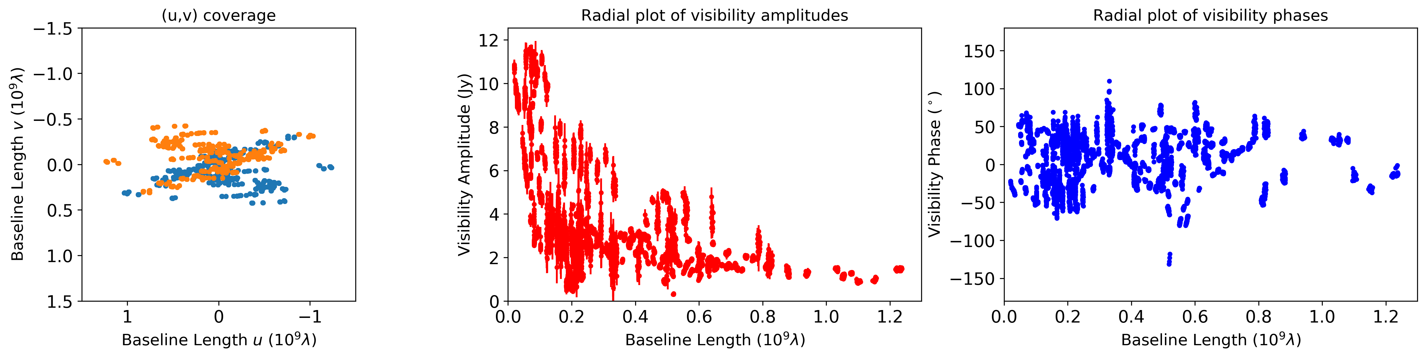
uvdata.VisTable has simple plot methods uvplot and raplot for plotting uv-coverages and radial plots. Each function is mocking pyploy.plot or pyplot.errorbar functions, and you can use almost all of arguments for pyplot.plot or pyplot.errorbar.
[19]:
# You can check fundamental properties of observations and visibilities
util.matplotlibrc(ncols=3, width=500, height=300)
fig, axs = plt.subplots(ncols=3)

plt.sca(axs[0])
plt.title("(u,v) coverage")
vtable.uvplot()
plt.xlim(1.5,-1.5)
plt.ylim(1.5,-1.5)

plt.sca(axs[1])
plt.title("Radial plot of visibility amplitudes")
vtable.radplot(datatype="amp",color="red")

plt.sca(axs[2])
plt.title("Radial plot of visibility phases")
vtable.radplot(datatype="phase",color="blue")
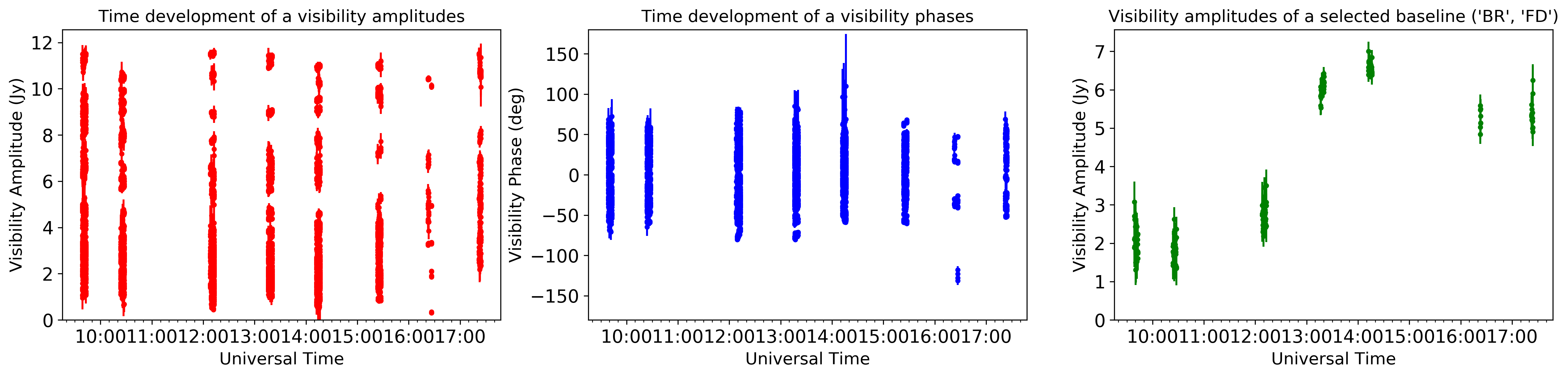
uvdata.VisTable has more flexible plotter vplot for various combination of data types. Available types of data are [“utc”,”gst”,”amp”,”phase”,”sigma”,”real”,”imag”,”u”,”v”,”uvd”,”snr”].
In this example, we show the utc time dependence of visibilities. You can also pick up a certain baseline information, where the available baselines are confirmed by vtable.baseline_list function.
[20]:
util.matplotlibrc(ncols=3, width=500, height=300)
fig, axs = plt.subplots(ncols=3)

plt.sca(axs[0])
plt.title("Time development of a visibility amplitudes")
vtable.vplot(axis1="utc",axis2="amp",color="red")

plt.sca(axs[1])
plt.title("Time development of a visibility phases")
vtable.vplot(axis1="utc",axis2="phase",color="blue")

plt.sca(axs[2])
plt.title("Visibility amplitudes of a selected baseline ('BR', 'FD')")
vtable.vplot(axis1="utc",axis2="amp",baseline=('BR', 'FD'),color="green")
plt.show()

# By the way, you can get the list of baselines by
baseline_list = vtable.baseline_list()
2.3.3. Make tables for bispectra and log closure amplitudes
From uvdata.VisTable, you can make tables for closure quantities such as bispectra (uvdata.BSTable) and log closure amplitudes (uvdata.CATable). The classes of both table also inherit pandas.DataFrame class, so you can use this class like pandas.DataFrame.
[21]:
# Calculate bispectra from vistable.VisTable objects
btable = vtable.make_bstable()
#btable = vtable.make_bstable(redundant=[["AA", "AP"], ["JC", "SM"]])  # removing trivial closure quatitites if the array has a redundant site

# Calculate log closure amplitudes from vistable.VisTable objects
ctable = vtable.make_catable()
#ctable = vtable.make_catable(redundant=[["AA", "AP"], ["JC", "SM"]])  # removing trivial closure quatitites if the array has a redundant site
2%|▏ | 141/7647 [00:00<00:05, 1401.74it/s]
(1/5) Sort data
(2/5) Tagging data
100%|██████████| 7647/7647 [00:05<00:00, 1326.31it/s]
 21%|██        | 51/248 [00:00<00:00, 505.69it/s]
  Number of Tags: 248
(3/5) Checking Baseline Combinations
100%|██████████| 248/248 [00:00<00:00, 565.98it/s]
  0%|          | 1/248 [00:00<00:31,  7.80it/s]
  Detect 25 combinations for Closure Phases
(4/5) Forming Closure Phases
100%|██████████| 248/248 [00:28<00:00,  8.66it/s]
  0%|          | 0/7647 [00:00<?, ?it/s]
(5/5) Creating BSTable object
(1/5) Sort data
(2/5) Tagging data
100%|██████████| 7647/7647 [00:05<00:00, 1287.45it/s]
 11%|█         | 27/248 [00:00<00:00, 242.35it/s]
  Number of Tags: 248
(3/5) Checking Baseline Combinations
100%|██████████| 248/248 [00:00<00:00, 478.10it/s]
  0%|          | 1/248 [00:00<00:37,  6.54it/s]
  Detect 25 combinations for Closure Amplitudes
(4/5) Forming Closure Amplitudes
100%|██████████| 248/248 [00:35<00:00, 18.17it/s]
(5/5) Creating CATable object
Data saving/loading funcitons are simiar to uvdata.VisTable.
[22]:
# Save
btable.to_csv("cphase.csv")
ctable.to_csv("logcamp.csv")

# Load
btable = uvdata.read_bstable("cphase.csv")
ctable = uvdata.read_catable("logcamp.csv")
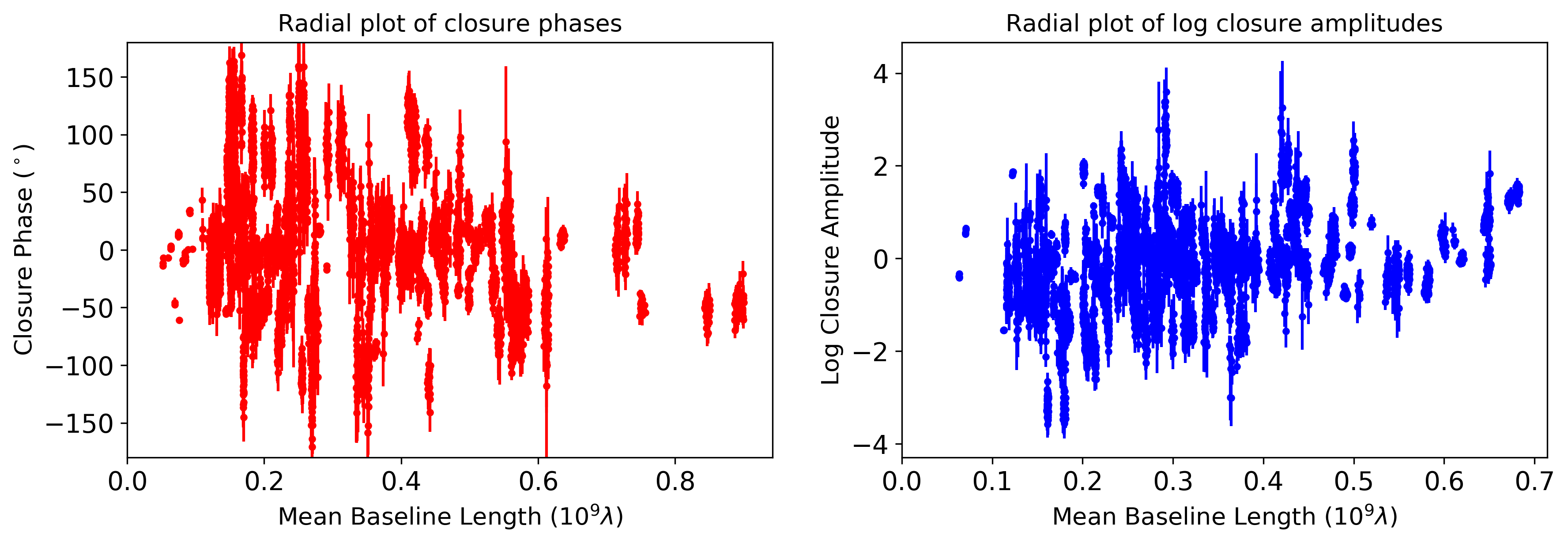
You can plot fundamental properties of observations and closure values.
[23]:
util.matplotlibrc(ncols=2, width=500, height=300)
fig, axs = plt.subplots(ncols=2)

plt.sca(axs[0])
plt.title("Radial plot of closure phases")
btable.radplot(color="red")

plt.sca(axs[1])
plt.title("Radial plot of log closure amplitudes")
ctable.radplot(color="blue")
plt.show()
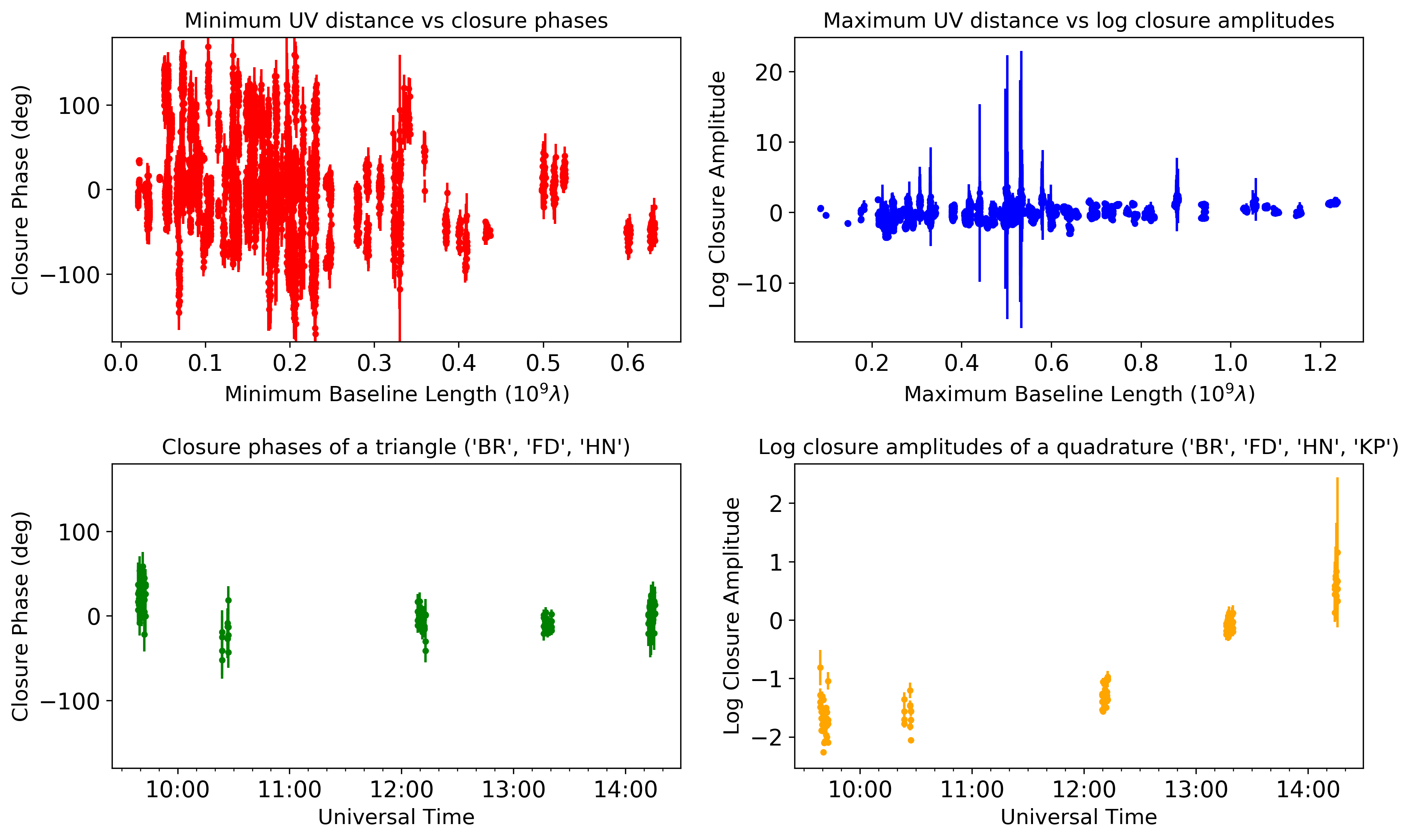
uvdata.BSTable and uvdata.CATable have vplot methods similar to uvdata.VisTable.
[24]:
util.matplotlibrc(nrows=2,ncols=2, width=500, height=300)
fig, axs = plt.subplots(nrows=2,ncols=2, sharex=False, sharey=False)
plt.subplots_adjust(hspace=0.4)

plt.sca(axs[0,0])
plt.title("Minimum UV distance vs closure phases")
btable.vplot(axis1="uvdmin", axis2="phase", color="red")

plt.sca(axs[0,1])
plt.title("Maximum UV distance vs log closure amplitudes")
ctable.vplot(axis1="uvdmax", axis2="logamp", color="blue")

plt.sca(axs[1,0])
plt.title("Closure phases of a triangle ('BR', 'FD', 'HN')")
btable.vplot(axis1="utc", axis2="phase", triangle=('BR', 'FD', 'HN'),color="green")

plt.sca(axs[1,1])
plt.title("Log closure amplitudes of a quadrature ('BR', 'FD', 'HN', 'KP')")
ctable.vplot(axis1="utc", axis2="logamp", quadrature=('BR', 'FD', 'HN', 'KP'),color="orange")
plt.show()

# By the way, you can get the combinations of baselines by
triangle_list = btable.triangle_list()
quadrature_list = ctable.quadrature_list()
2.3.4. Acknowledgement
This notebook makes use of 43 GHz VLBA data from the VLBA-BU Blazar Monitoring Program (VLBA-BU-BLAZAR; http://www.bu.edu/blazars/VLBAproject.html), funded by NASA through the Fermi Guest Investigator Program. The VLBA is an instrument of the National Radio Astronomy Observatory. The National Radio Astronomy Observatory is a facility of the National Science Foundation operated by Associated Universities, Inc.