2.2. Image regions

In interferometric imaging or any image processing, often we need to set regions where the intensity will be solved or to mask images. SMILI provide a class for handling geometric description of such regions.

This notebook provides an example usage how to read, set and save image regions.

%matplotlib inline
from pylab import *
from smili import imdata, util

An instance of ds9 was found to be running before we could
start the 'xpans' name server. You will need to perform a
bit of manual intervention in order to connect this
existing ds9 to Python.

For ds9 version 5.7 and beyond, simply register the
existing ds9 with the xpans name server by selecting the
ds9 File->XPA->Connect menu option. Your ds9 will now be
fully accessible to pyds9 (e.g., it appear in the list
returned by the ds9_targets() routine).

For ds9 versions prior to 5.7, you cannot (easily) register
with xpans, but you can view ds9's File->XPA Information
menu option and pass the value associated with XPA_METHOD
directly to the Python DS9() constructor, e.g.:

    d = DS9('a000101:12345')

The good news is that new instances of ds9 will be
registered with xpans, and will be known to ds9_targets()
and the DS9() constructor.

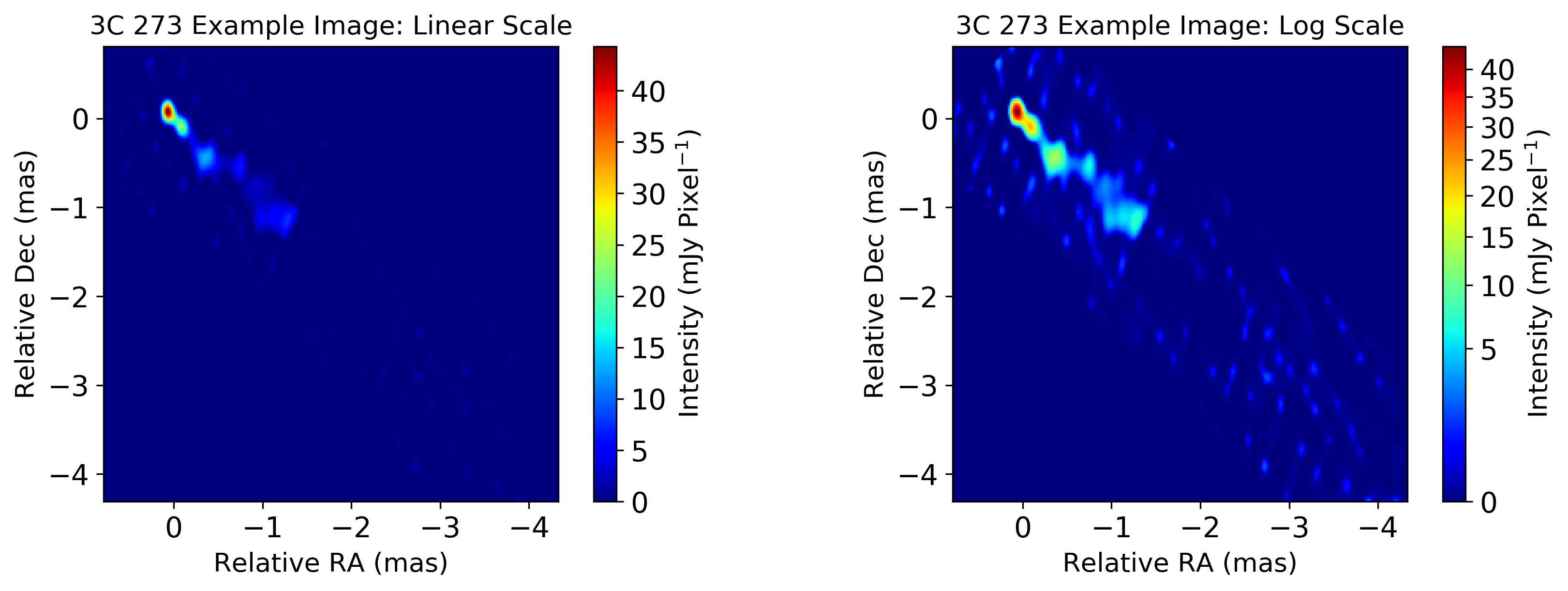
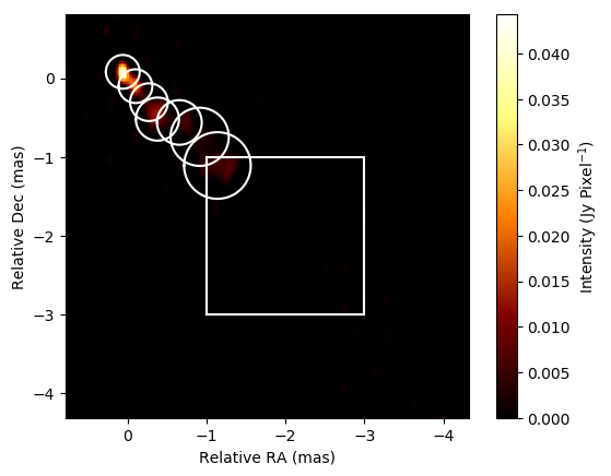
Here, we use an FITS image reconstructed with SMILI from a 43 GHz 3C 273 data set of the Boston University Blazar Group.

# Load the FITS image
image = imdata.IMFITS("./BU_3C273_sampleimage.fits", angunit="mas")

# Plot the image in linear and log scales
util.matplotlibrc(ncols=2, width=500, height=300)
fig, axs = plt.subplots(ncols=2)

plt.sca(axs[0])
plt.title("3C 273 Example Image: Linear Scale")
image.imshow(colorbar=True, fluxunit="mjy", cmap=cm.jet)

plt.sca(axs[1])
plt.title("3C 273 Example Image: Log Scale")
image.imshow(scale="gamma", fluxunit="mjy", colorbar=True, cmap=cm.jet)

mpl.rcdefaults()

2.2.1. Interactively set imaging regions using SAO DS9

SMILI can intractively set regions with SAO DS9 using pyds9. To load your image to DS9, you can use open_pyds9 method of your image object.

# Open this image in DS9
image.open_pyds9()

Or alternatively, you can create a imdata.IMRegion object and use open_pyds9 method.

# Initialize an IMRegion object
imregion = imdata.IMRegion()

# Open the image in DS9. If this imregion has already some regions, it will be sent to DS9 as well.
imregion.open_pyds9(image)

You can see your image in DS9 and set regions.

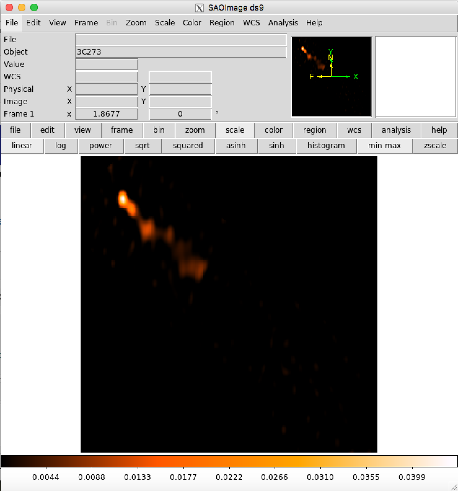
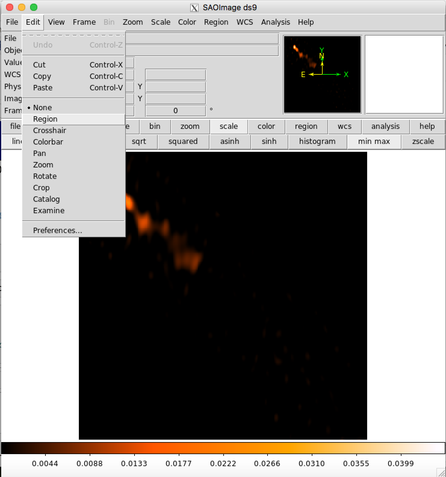
You can set a region by clicking EDIT > Region. Currently, SMILI can handle circles, squares and ellipses in DS9. Here, ellipses are set to the area with significant flux densities.

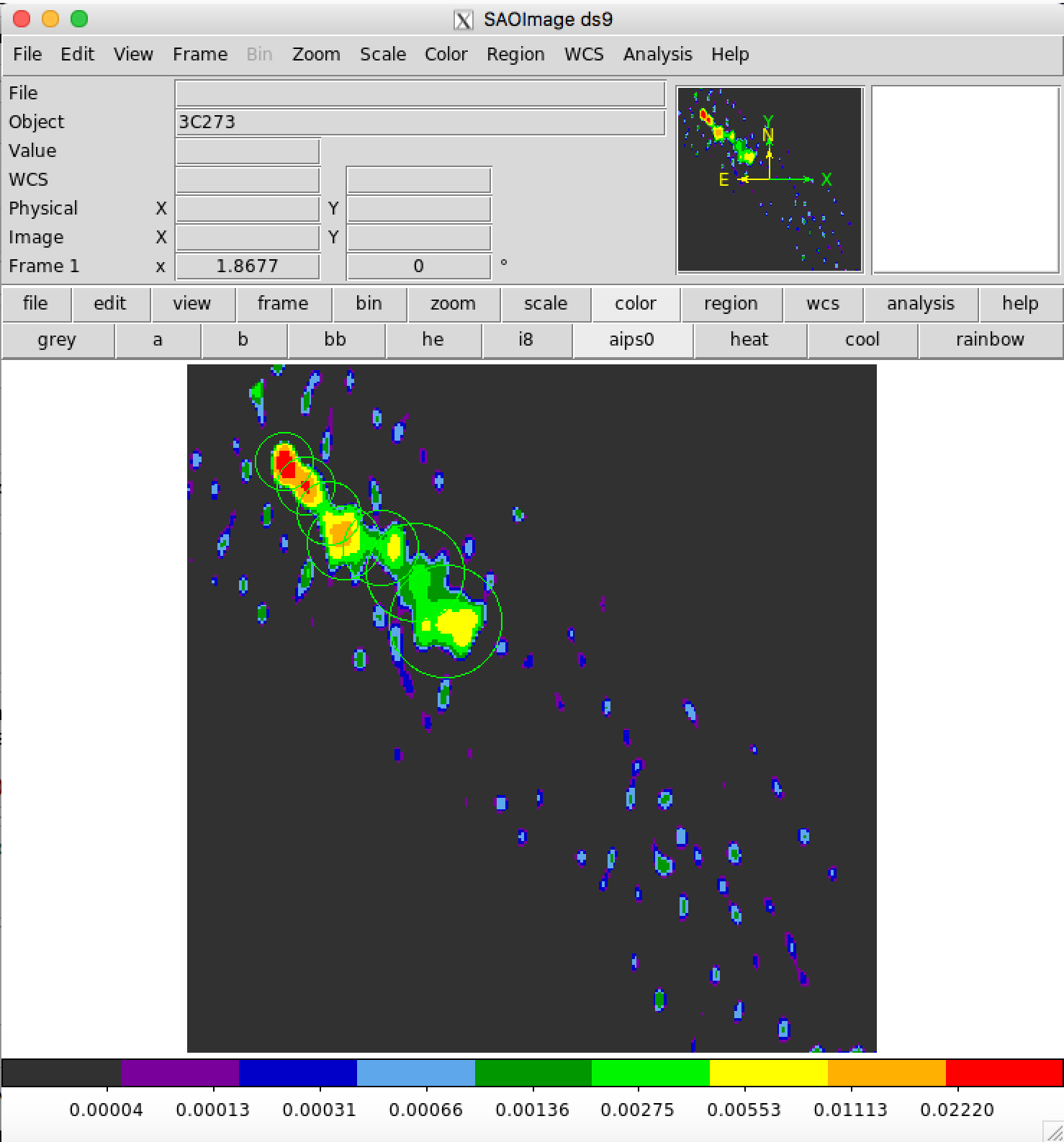
You can pull regions from DS9 with load_pyds9 methods in imdata.IMFITS or imdata.IMRegion objects.

# eighther of commands will work to pull regions from DS9
imregion = image.load_pyds9()
imregion = imregion.load_pyds9(image)

The imdata.IMRegion class is inheriting pandas.DataFrame. You can use all functions available for pandas.DataFrame.

imregion

	shape	xc	yc	width	height	radius	maja	mina	angle	angunit
0	circle	61.83334	80.4166	NaN	NaN	214.16716	NaN	NaN	NaN	uas
1	circle	-98.79166	-101.6250	NaN	NaN	214.16716	NaN	NaN	NaN	uas
2	circle	-270.12500	-305.0834	NaN	NaN	239.36694	NaN	NaN	NaN	uas
3	circle	-377.20834	-519.2500	NaN	NaN	273.55490	NaN	NaN	NaN	uas
4	circle	-655.62500	-562.0834	NaN	NaN	283.40834	NaN	NaN	NaN	uas
5	circle	-912.62500	-744.1250	NaN	NaN	369.12282	NaN	NaN	NaN	uas
6	circle	-1137.50000	-1108.2084	NaN	NaN	422.75350	NaN	NaN	NaN	uas

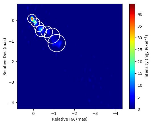
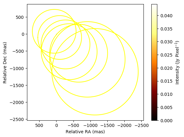
In addition, it has additional functions. For instance, you can plot your regions with plot method.

# plot the original image as a reference
image.imshow(colorbar=True, fluxunit="mjy", cmap=cm.jet)

# plot regions. You can use any arguments of pyplot.plot for customizing your plots.
imregion.plot(color="white", angunit="mas")

You can save this region file to a csv file with to_csv method, and load it again with imdata.read_imregion function

# save this region file to a csv file
imregion.to_csv("imregion.csv")

# load this region file from the csv file
imregion = imdata.read_imregion("imregion.csv")

If you have a pixel-coordinated DS9 region file, you can also read it with load_ds9reg method

# Load DS9 region file (must be using pixel-based coordinates)
imregion_ds9 = imdata.IMRegion()
imregion_ds9 = imregion_ds9.load_ds9reg(regfile="xxx.reg",image=image)

2.2.2. Manually set/edit imaging regions

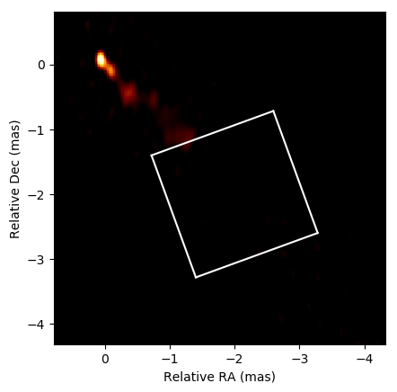
You can also add regions from SMILI. This would be useful to pipeline imaging scripts.

# Adding a box
imregion_box = imdata.IMRegion()
imregion_box= imregion_box.add_box(xc=-2,yc=-2,width=2,angle=20,angunit="mas")

# Check
image.imshow()
imregion_box.plot(color="white")

# Adding a circle
imregion_circ = imdata.IMRegion()
imregion_circ= imregion_circ.add_circle(xc=0,yc=0,radius=0.5,angunit="mas")

# Check
image.imshow()
imregion_circ.plot(color="white")

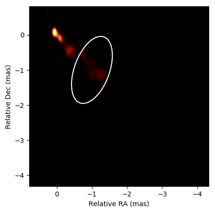
# Adding a circle
imregion_ellip = imdata.IMRegion()
imregion_ellip = imregion_ellip.add_ellipse(xc=-1,yc=-1,maja=2,mina=1,angle=20,angunit="mas")

# Check
image.imshow()
imregion_ellip.plot(color="white")

There are some other useful functions to edit regions

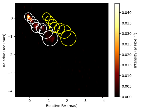
# Shifting imaging regions.
imregion_shift = imregion.copy()
imregion_shift.shift(dx=-1,dy=0,angunit="mas")

# Check
image.imshow(colorbar=True)
imregion.plot(color="white", label="original", angunit="mas")
imregion_shift.plot(color="yellow", label="shifted", angunit="mas")

# Zoom regions
imregion_zoom = imregion.copy()
imregion_zoom.zoom(fx=3)

# Check
image.imshow(colorbar=True)
imregion.plot(color="white", label="original")
imregion_zoom.plot(color="yellow")

You can also add regions.

Create region1 and region2.

# Create two imaging regions
imregion1 = imregion.copy()
imregion2 = imdata.IMRegion().add_box(xc=-2,yc=-2,width=2,angle=0,angunit="mas")

# Take a sum
imregion3 = imregion1 + imregion2

# Check
image.imshow(colorbar=True)
imregion3.plot(color="white", angunit="mas")

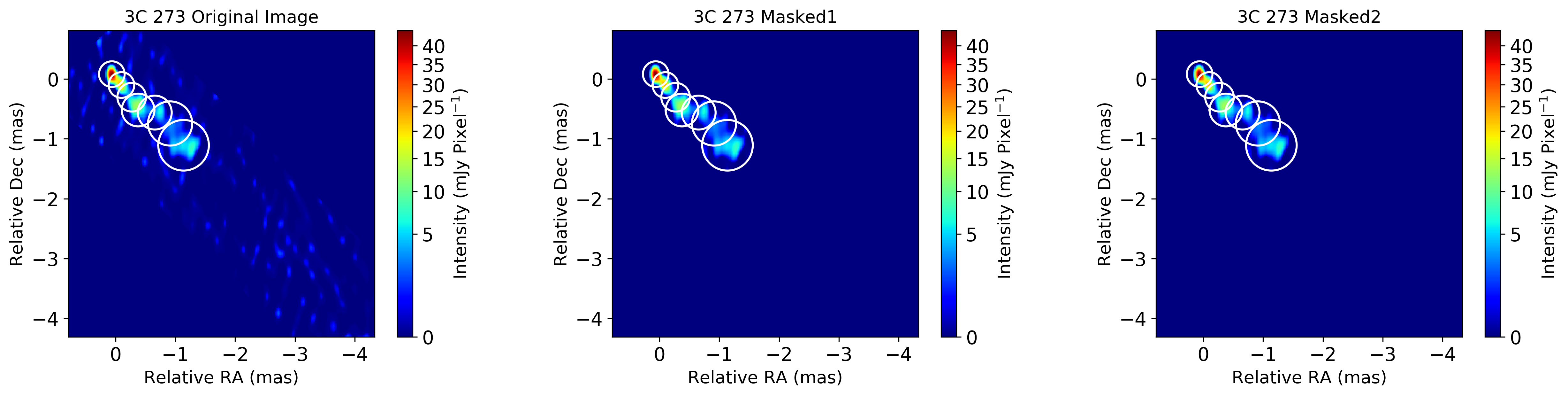
2.2.3. Masking image with imregion

You can mask images with winmod methods in imdata.IMFITS/imdata.IMRegion objects.

# These commands are equivalent
editimage1 = imregion.winmod(image,save_totalflux=False)
editimage2 = image.winmod(imregion, save_totalflux=False)

# Check: indeed you can see all brightness outside regions are cleared.
util.matplotlibrc(ncols=3, width=500, height=300)
fig, axs = plt.subplots(ncols=3)

plt.sca(axs[0])
plt.title("3C 273 Original Image")
image.imshow(scale="gamma",  fluxunit="mjy", colorbar=True,cmap=cm.jet)
imregion.plot(color="white", angunit="mas")

plt.sca(axs[1])
plt.title("3C 273 Masked1")
editimage1.imshow(scale="gamma", fluxunit="mjy", colorbar=True, cmap=cm.jet)
imregion.plot(color="white", angunit="mas")

plt.sca(axs[2])
plt.title("3C 273 Masked2")
editimage2.imshow(scale="gamma", fluxunit="mjy", colorbar=True, cmap=cm.jet)
imregion.plot(color="white", angunit="mas")

mpl.rcdefaults()

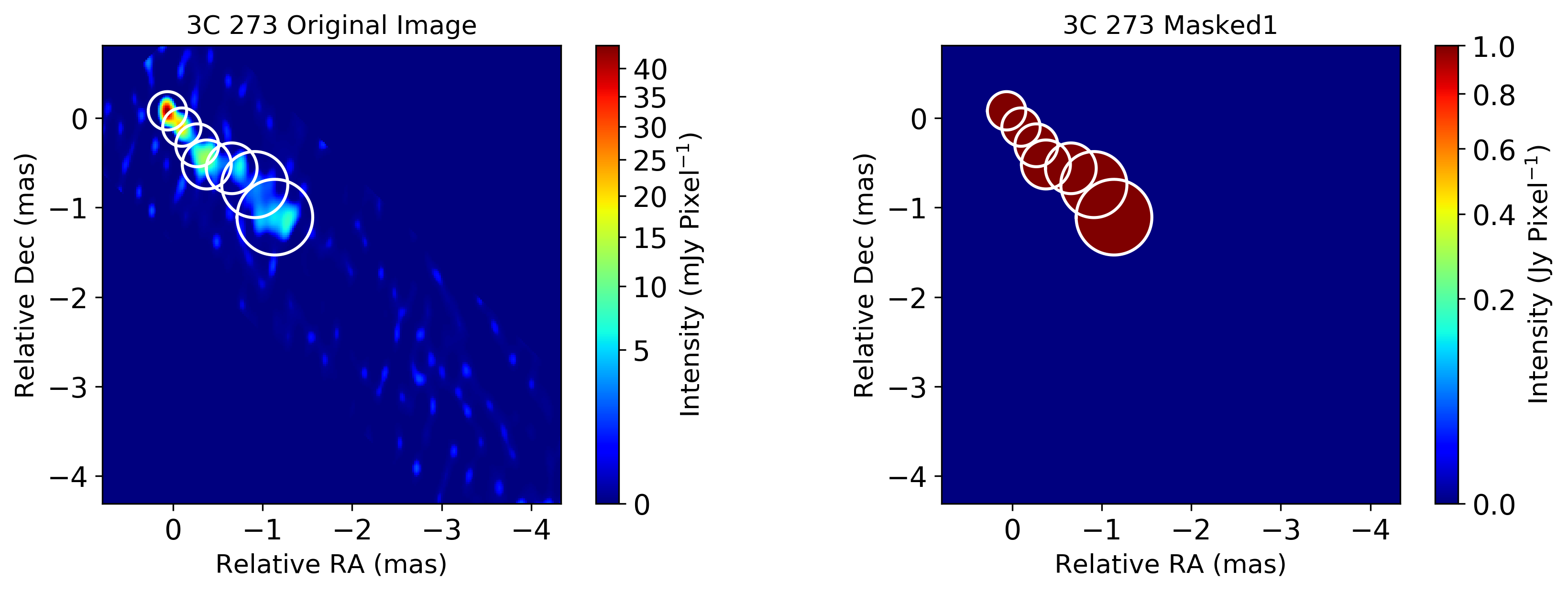
You can also creat a “mask image”, which can be loaded to imaging functions as well

# Create a mask image
maskimage = imregion.maskimage(image)

# Check: indeed you can see all brightness outside regions are cleared.
util.matplotlibrc(ncols=2, width=500, height=300)
fig, axs = plt.subplots(ncols=2)

plt.sca(axs[0])
plt.title("3C 273 Original Image")
image.imshow(scale="gamma",  fluxunit="mjy", colorbar=True,cmap=cm.jet)
imregion.plot(color="white", angunit="mas")

plt.sca(axs[1])
plt.title("3C 273 Masked1")
maskimage.imshow(scale="gamma", colorbar=True, cmap=cm.jet)
imregion.plot(color="white", angunit="mas")

mpl.rcdefaults()

2.2.4. Acknowledgement

This notebook makes use of 43 GHz VLBA data from the VLBA-BU Blazar Monitoring Program (VLBA-BU-BLAZAR; http://www.bu.edu/blazars/VLBAproject.html), funded by NASA through the Fermi Guest Investigator Program. The VLBA is an instrument of the National Radio Astronomy Observatory. The National Radio Astronomy Observatory is a facility of the National Science Foundation operated by Associated Universities, Inc.